
Q1. What are some ways to check the normality of a data?
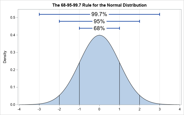
Way 1: Visualize it! If you plot a histogram of all the data points available, it should look similar to following curve (All the curves are normally distributed, they just have different means and standard deviations).

This curve is called a Bell Shaped Curve, meaning:
- 68% of the values are found within 1 Standard Deviation away from the mean
- 95% of the values are found within 2 Standard Deviations away from the mean
- 99.7% of the values are found within 3 Standard Deviations away from the mean
Way 2: Test it with a statistical test. One of the most common test is Anderson Darling test for normality. The test assumes the following hypothesis:
- Ho = The data is normally distributed
- Ha = The data is not normally distributed
In python you can use this test with following piece of code:
scipy.stats.anderson(x, dist='norm')
The result may look something like:AndersonResult(statistic=1.383562257554786,critical_values=array([0.574, 0.654, 0.785, 0.916, 1.089]), significance_levelsignificance_level=array([15. , 10. , 5. , 2.5, 1. ]))
In order to reject the NULL hypothesis, the test statistic should be larger than any given critical value. In this case it is larger than all the critical values, so we can say with 99% confidence that the distribution is not normally distributed.
Other tests:
scipy.stats.normaltest(a, axis=0, nan_policy='propagate')scipy.stats.shapiro(x)
NOTE: All of them have the same null hypothesis.
2. What are the key assumptions for Linear Regression?
There are following assumptions associated with it:
- Linearity: The relationship between dependent and independent variable is linear
- Independence: All the observations (rows) in the dataset are independent of each other
- Normality: For any fixed value of independent variable, the dependent variable follows a normal distribution
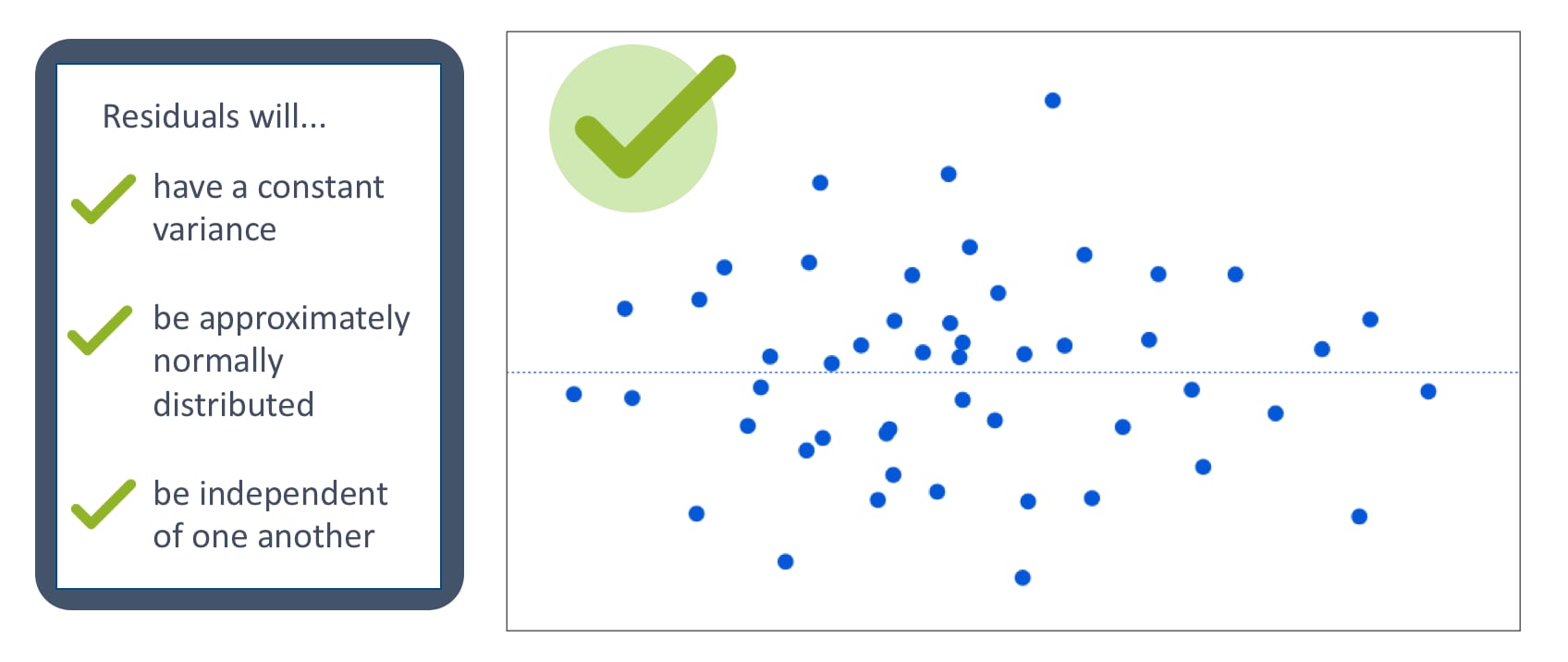
- Homoscedasticity: The residuals are randomly distributed around it's mean
- No multicollinearity: The is NO or very little correlation between the independent variables
- No autocorrelation: This means that the residuals are not dependent on each other

You can also check it out in this article, if you are working in R:
3. What are the assumptions for Logistic Regression?
- Independence: Same as above
- No Multicollinearity: Same as above
- Linearity: Here, is assumes that the independent variable has a linear relationship with the log odds of the dependent variable
- Large sample size: Rule of thumb is that we need at least 10 observations for the least frequent outcome for each independent variable. For example, if we have 10 independent variables and the probability of the least frequent outcome is 0.5, the we need 10*10/0.5 = 200 observations
4. What is Multicollinearity and how do we fix it?
So here's the thing, the key assumption for a linear regression is that we need to isolate the relationship between each independent variable and the dependent variable. Regression coefficient represents the mean change in dependent variable with one unit change in the independent variable, while keeping all other independent variables constant. Now, here's why this is important!
When you try to change an independent variable by 1 unit to model the mean change in dependent variable, it becomes difficult to isolate it when the independent variables are correlated. Higher the correlation is, more they'll change with one unit change in one of them. So, it becomes difficult for the model to estimate the change in dependent variable by a single independent variable since there's another independent variable moving in unison. So, we can't afford to have it.
Also, there are two type of multicollinearity:
- Structural: This may come up in your data when you create interaction terms
- Data: This is already present in the default dataset available to us
What do we do to fix it?
Variation Inflation Factor (VIF) Analysis
VIF determines the correlation and strength of correlations between the independent variables.
- VIF = 1, no correlation at all (VIF starts at 1)
- VIF between 1 and 5, low to moderate correlation, but not strong enough to do anything about it
- VIF > 5, you need to remove them to reduce multicollinearity
To reduce structural multicollinearity, you can center the independent variable before using in the regression. This means that you can standardize in any way (one of the ways is to calculate the mean of the columns and take a difference of each value with the mean to make it centered around the mean). This will reduce the structural multicollinearity significantly.
5. What is the relationship between VIF and Tolerance?
Tolerance = 1-R^2
This means that we need to have higher Tolerance in order to have low multicollinearity. This is quite intuitive.
VIF = 1/Tolerance
VIF is the quotient of the variance in a model with multiple terms with variance of a model with only one term. It provides an index of measure that explains how much variance of an estimated regression coefficient is increased due to presence of multicollinearity.
NOTE: VIF is a method to quantify the severity of multicollinearity in OLS regression analysis
6. Which one treat first: missing values or outliers?
In my opinion, it is important to deal with the outliers first. Why? Here's the thing, consider you have a column 'Age' and you have values from 1 to 100 along with an outlier which it 450. Now there's a high chance that this is just a typing mistake where the person entering the age wanted to enter 45, but added a 0 by mistake.
You might figure it out using other independent variables in the dataset, like 'Salutation', 'Weight', 'Current occupation' etc.
Imagine not handling this first and trying to figure out the missing values in the dataset. If you end up replacing the missing values with the mean of the age column (the simplest technique), you'll count 450 into that and the overall mean will be more than it should be. Which might not be a good estimation and your data becomes biased.
Please put down your thoughts in the comments! I'd like to see your opinion.
7. What do you mean by Sensitivity and Specificity?
I'll go ahead an explain the whole confusion matrix in this question so that we're done once and for all.

The above is a confusion matrix. You all should be familiar with that! Now there are few key terminologies that you should know here:
- Classification Rate or Overall Accuracy = (TP + TN) / (TP + TN + FP + FN)
However, this may not be the best parameter to look at in all the cases. That's because it's giving equal penalties to both kinds of errors (FN and FP)
- Recall = TP / (TP + FN) = TP / Actual Positives
This is intuitive enough. This is the ratio of correctly predicted class over overall actual positives. Higher the recall, high the number of correct classifications done by the model
NOTE: this is also known as SENSITIVITY or a TRUE POSITIVE RATE
- Precision = TP / (TP + FP) = TP / Predicted Positives
Again, this is the ratio of correctly predicted positives over the total predicted positives. Higher precision indicates that from the total predicted positives, there's a high number of actual positives.
- Specificity = TN / (TN + FP)
This is also known as TRUE NEGATIVE RATE and means that the proportional of true negative predicted over the total actual negatives in the dataset
A few cases you might come across:
High recall and low precision: This means that most of the positive class is correctly predicted by the model (low FN), but there are a lot of false positives.
Low recall and high precision: This shows that we failed to predict a lot of positives (high FN) but whatever we are predicting as positive are actually positive (low FP)
I'll write another article with more questions!
Cheers!
Nitin
Thank you Nitin. This was quite useful, waiting for more blogs like these !
ReplyDeleteI'm glad you like it!
Delete