
Those who ended up directly on this part, please use this link to read Part 1 and come back to this.
5. Removing trend and seasonality
One of the easiest ways to REDUCE, not REMOVE trend from the time series is to transform it so that the higher values are penalised more than the smaller values. There are many ways to do it, log transformation, square root, cube root transformation etc. You can try them on your time series to see what makes the most sense. In our case, though, there don't seem to be a visible overall trend. But we will still do ahead and try to do these transformations and see what happens:


Doesn't change much except the scale, does it? Let's keep the original then.
We can use some techniques to estimate or model the trend from the time series and then remove it. The most common one is called 'SMOOTHING'. Smoothing is nothing but taking rolling estimates (like moving average, weighted moving average etc.) and then subtract it from the actual value to get the residual series.
Moving Average
Let's try to do the Moving Average (btw, we see moving averages a lot in stock pricing websites). I'm taking the moving average of last 90 days. You can try and change it to see what difference does it make:
# rolling mean
ma90 = daily_energy_data.rolling(90).mean()
figure(num=None, figsize=(20, 5), dpi=80, facecolor='w', edgecolor='k')
plt.plot(daily_energy_data)
plt.plot(ma90)

Now let's take the difference of the moving average value with the actual value. NOTE that you'll not get any value for the first 90 days as there's no moving average value corresponding to them. After taking the difference, we will test for stationarity again using our rolling_stats() and dickey_fuller() function:
ma_diff = daily_energy_data - ma90
ma_diff.dropna(inplace=True)
rolling_stats(ma_diff)

There sure is a little improvement if you compare it with the test results on the original data. Now let's do the Dickey Fuller test:
dicky_fuller(ma_diff)
Dickey-Fuller Test Results:
Test Statistic                  -2.803916
p-value                          0.057717
#Lags Used                      10.000000
Number of Observations Used    572.000000
Critical Value (1%)             -3.441834
Critical Value (5%)             -2.866606
Critical Value (10%)            -2.569468
dtype: float64
The results shows that the Test Statistic is larger than all the Critical values, and the p-value is > 0.05. So we're not quite there yet. Let's try another technique.
Exponential Weighted Average
expwighted_avg = daily_energy_data.ewm(com=12).mean()
figure(num=None, figsize=(20, 5), dpi=80, facecolor='w', edgecolor='k')
plt.plot(daily_energy_data)
plt.plot(expwighted_avg)

de_data_ewma_diff = daily_energy_data - expwighted_avg
rolling_stats(de_data_ewma_diff)

Much much better than before. Let's check the Dickey Fuller test results:
dicky_fuller(de_data_ewma_diff)
Dickey-Fuller Test Results:
Test Statistic                -1.782706e+01
p-value                        3.144223e-30
#Lags Used                     0.000000e+00
Number of Observations Used    6.710000e+02
Critical Value (1%)           -3.440133e+00
Critical Value (5%)           -2.865857e+00
Critical Value (10%)          -2.569069e+00
dtype: float64
These are all simple techniques to reduce stationarity in your time series. But they may not work very well in cases where you have high seasonality. In order to reduce trend and seasonality there, we can use following 2 techniques:
- Differencing
- Decomposition
Differencing
Differencing means that you make a new series which is = Series(t) - Series(t-n). This is the most commonly used way of dealing with trend and seasonality. When n = 1, its called First Order Differencing. When n = 2, its called Second Order Differencing and so on. Let's do a First Order Differencing:
de_data_diff = daily_energy_data - daily_energy_data.shift()
figure(num=None, figsize=(20, 5), dpi=80, facecolor='w', edgecolor='k')
plt.plot(de_data_diff)

This seem to have reduced trend and stationarity real good. Let's test it out with rolling_stats() and dickey_fuller()
de_data_diff.dropna(inplace=True)
rolling_stats(de_data_diff)

This one's look great. Do you see how mean is so constant here?
dicky_fuller(de_data_diff)Dickey-Fuller Test Results: Test Statistic -1.160513e+01 p-value 2.592066e-21 #Lags Used 1.200000e+01 Number of Observations Used 6.580000e+02 Critical Value (1%) -3.440327e+00 Critical Value (5%) -2.865942e+00 Critical Value (10%) -2.569114e+00 dtype: float64
The Test Statistic and p-value are way under the thresholds. So differencing did a great job reducing trend and seasonality.
Decomposition
This is where the trend and seasonality are modelled separately and the residual series is returned. This residual series is supposed to be stationary and you can use statistical forecasting on that.daily_energy_data.reset_index(inplace=True)
daily_energy_data['date'] = pd.to_datetime(daily_energy_data['date'])
daily_energy_data = daily_energy_data.set_index('date')
from statsmodels.tsa.seasonal import seasonal_decompose
decomposition = seasonal_decompose(daily_energy_data)
trend = decomposition.trend
seasonal = decomposition.seasonal
residual = decomposition.resid
fig, ax = plt.subplots(4,1, figsize=(15,15))
ax[0].plot(daily_energy_data, label='Original')
ax[0].legend(loc='best')
ax[1].plot(trend, label='Trend')
ax[1].legend(loc='best')
ax[2].plot(seasonal,label='Seasonality')
ax[2].legend(loc='best')
ax[3].plot(residual, label='Residuals')
ax[3].legend(loc='best')
fig.tight_layout()


residual.dropna(inplace=True)
rolling_stats(residual)

dicky_fuller(residual)Dickey-Fuller Test Results: Test Statistic -1.167763e+01 p-value 1.772417e-21 #Lags Used 2.000000e+01 Number of Observations Used 6.450000e+02 Critical Value (1%) -3.440529e+00 Critical Value (5%) -2.866031e+00 Critical Value (10%) -2.569162e+00 dtype: float64
Similar results, right?
6. Time series forecasting techniques
We will go ahead and use the differencing series for forecasting as it is one of the most commonly used technique.
- AR or Autoregressive Model
In this method, the we model the next step in the time series as a linear function of observations at any previous steps. Here, you're supposed to tell the order of the model, i.e. how many previous lagged values are you considering.
An AR model is denoted as AR(p) where p is the order of the model. If the order is 1, then AR(1):
yt = bo + b1*yt-1 + et
yt = bo + b1*yt-1 + b2*yt-2 + et
and so on...
This model is based on the assumption of AUTOCORRELATION. What it means is that a variable at any time is correlated with its own values at previous time intervals. The correlation can either be positive or negative. But since the correlation is with itself, it's called autocorrelation. Higher the correlation with a particular lagged value, the coefficient will get a higher weight in the linear equation of the AR(p) model.
You can use the following piece of code to implement AR model:
from statsmodels.tsa.ar_model import AutoReg
from random import random
data = <your_dataframe>
p = <the_order>Now we need to know how do we define the order of an autoregressive model. We do that by using PACF plot or Partial Autocorrelation Function.
# fit model
model = AutoReg(data, lags=p)
model_fit = model.fit()
# make prediction
yhat = model_fit.predict(len(data), len(data))
print(yhat)
What is PACF?
PACF determines only the direct correlation between a value at time t and a value at time t-k for the variable. PACF tends to remove all other correlations that are explained by the ACF due to the effects of other values at times in between t and t-k.
import statsmodels.api as sm
fig = sm.graphics.tsa.plot_pacf(de_data_diff.daily_energy.squeeze(), lags=20)

Now, in our case, we see that there are 6 lags which are above the confidence level. So we will use the AR order 'p' as 6.
- MA or Moving Average Model
Now, this is not just a simple moving average that we can plot using the rolling mean.
As we saw in the AR model, it uses previous values of the same variable to forecast a value at time t, in MA model, instead of using the values, it uses the error between the actual and predicted values in the past to forecast the value at time t.
yt=c+εt+θ1εt−1+θ2εt−2+⋯+θqεt−q
Here also, we need to identify the order of the MA model and that is defined by 'q'. We find the order by using the ACF plot!
What is ACF plot?
The ACF plot not only includes the direct correlation of y at time t with y at time t - k but it also includes the effects of correlations due to all the time lags in between that period. This gives us the whole package!
fig = sm.graphics.tsa.plot_acf(de_data_diff.daily_energy.squeeze(), lags=20)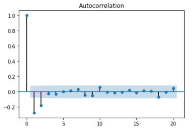
- ARMA Model
Now it's pretty clear that this model is a mix of both the AR and the MA model. Hence it models the next value as a linear function of values and residual errors in the previous steps or time periods. Its notation is ARMA(p, q) as it will take orders of both the AR and MA models.
- ARIMA Model
The I in ARIMA is 'Integrated'. It models the next value as a linear function of differenced values and residual errors in the previous steps or time periods. Its notation is ARMA(p, d, q) as it will take orders of both the AR and MA models along with the differencing pre-processing step of the sequence to make the sequence stationary.
Now here's the thing about differencing. We already did this steps previously and have been using the 1st order differenced series in ACF and PACF. So we can either set d = 0 here or use the original series and set d = 1 here.
7. Forecasting a time series
Let's use ARIMA model to model all the above models we discussed.
from statsmodels.tsa.arima_model import ARIMA
# AR Model
model = ARIMA(de_data_diff, order=(6, 0, 0))
results_AR = model.fit(disp=-1)
figure(num=None, figsize=(20, 5), dpi=80, facecolor='w', edgecolor='k')
plt.plot(de_data_diff)
plt.plot(results_AR.fittedvalues, color='red')
plt.title('RSS: %.4f'% sum((results_AR.fittedvalues - de_data_diff.daily_energy)**2))

# MA Model
model = ARIMA(de_data_diff, order=(0, 0, 2))
results_AR = model.fit(disp=-1)
figure(num=None, figsize=(20, 5), dpi=80, facecolor='w', edgecolor='k')
plt.plot(de_data_diff)
plt.plot(results_AR.fittedvalues, color='red')
plt.title('RSS: %.4f'% sum((results_AR.fittedvalues - de_data_diff.daily_energy)**2))

# ARMA Model
model = ARIMA(de_data_diff, order=(4, 0, 2))
results_AR = model.fit(disp=-1)
figure(num=None, figsize=(20, 5), dpi=80, facecolor='w', edgecolor='k')
plt.plot(de_data_diff)
plt.plot(results_AR.fittedvalues, color='red')
plt.title('RSS: %.4f'% sum((results_AR.fittedvalues - de_data_diff.daily_energy)**2))

# ARIMA Model
model = ARIMA(daily_energy_data, order=(4, 1, 2))
results_AR = model.fit(disp=-1)
figure(num=None, figsize=(20, 5), dpi=80, facecolor='w', edgecolor='k')
plt.plot(de_data_diff)
plt.plot(results_AR.fittedvalues, color='red')
plt.title('RSS: %.4f'% sum((results_AR.fittedvalues - de_data_diff.daily_energy)**2))

Here you'll see that the ARMA and ARIMA models are exactly same. I made both of them to show you how you can do the differencing directly within the model itself.
Now the RSS of the AR model is the highest, then these is a significant reduction in RSS in MA model and then eventually a little reduction in ARMA/ARIMA model.
Now the only thing left is to bring it back to the original series. I think you can do that yourself and try to plot it!
Send back your feedback in comments!
Cheers!
Nitin.
Comments
Post a Comment